Cold Magnetized Plasma Waves Tensor Elements (S, D, P in Stix’s notation)

This example shows how to calculate the values of the cold plasma tensor elements for various electromagnetic wave frequencies.

# First, import some basics (and `PlasmaPy`!)
import numpy as np
import plasmapy as pp
import matplotlib.pyplot as plt
from astropy import units as u

Let’s define some parameters, such as the magnetic field magnitude, the plasma species and densities and the frequency band of interest

B = 2 * u.T
species = ['e', 'D+']
n = [1e18 * u.m ** -3, 1e18 * u.m ** -3]

f = np.logspace(start=6, stop=11.3, num=3001)  # 1 MHz to 200 GHz
omega_RF = f * (2 * np.pi) * (u.rad / u.s)

help(pp.physics.cold_plasma_permittivity_SDP)

Out:

Help on function cold_plasma_permittivity_SDP in module plasmapy.physics.dielectric:

cold_plasma_permittivity_SDP(B, species, n, omega)
    Magnetized Cold Plasma Dielectric Permittivity Tensor Elements.

    Elements (S, D, P) are given in the "Stix" frame, ie. with B // z.

    The :math:`\exp(-i \omega t)` time-harmonic convention is assumed.

    Parameters
    ----------
    B : ~astropy.units.Quantity
        Magnetic field magnitude in units convertible to tesla.

    species : list of str
        List of the plasma particle species
        e.g.: ['e', 'D+'] or ['e', 'D+', 'He+'].

    n : list of ~astropy.units.Quantity
        `list` of species density in units convertible to per cubic meter
        The order of the species densities should follow species.

    omega : ~astropy.units.Quantity
        Electromagnetic wave frequency in rad/s.

    Returns
    -------
    S : ~astropy.units.Quantity
        S ("Sum") dielectric tensor element.

    D : ~astropy.units.Quantity
        D ("Difference") dielectric tensor element.

    P : ~astropy.units.Quantity
        P ("Plasma") dielectric tensor element.

    Notes
    -----
    The dielectric permittivity tensor is expressed in the Stix frame with
    the :math:`\exp(-i \omega t)` time-harmonic convention as
    :math:`\varepsilon = \varepsilon_0 A`, with :math:`A` being

    .. math::

        \varepsilon = \varepsilon_0 \left(\begin{matrix}  S & -i D & 0 \\
                              +i D & S & 0 \\
                              0 & 0 & P \end{matrix}\right)

    where:

    .. math::
        S = 1 - \sum_s \frac{\omega_{p,s}^2}{\omega^2 - \Omega_{c,s}^2}

        D = \sum_s \frac{\Omega_{c,s}}{\omega}
            \frac{\omega_{p,s}^2}{\omega^2 - \Omega_{c,s}^2}

        P = 1 - \sum_s \frac{\omega_{p,s}^2}{\omega^2}

    where :math:`\omega_{p,s}` is the plasma frequency and
    :math:`\Omega_{c,s}` is the signed version of the cyclotron frequency
    for the species :math:`s`.

    References
    ----------
    - T.H. Stix, Waves in Plasma, 1992.

    Examples
    --------
    >>> from astropy import units as u
    >>> from plasmapy.constants import pi
    >>> B = 2*u.T
    >>> species = ['e', 'D+']
    >>> n = [1e18*u.m**-3, 1e18*u.m**-3]
    >>> omega = 3.7e9*(2*pi)*(u.rad/u.s)
    >>> S, D, P = cold_plasma_permittivity_SDP(B, species, n, omega)
    >>> S
    <Quantity 1.02422902>
    >>> D
    <Quantity 0.39089352>
    >>> P
    <Quantity -4.8903104>

S, D, P = pp.physics.cold_plasma_permittivity_SDP(B, species, n, omega_RF)

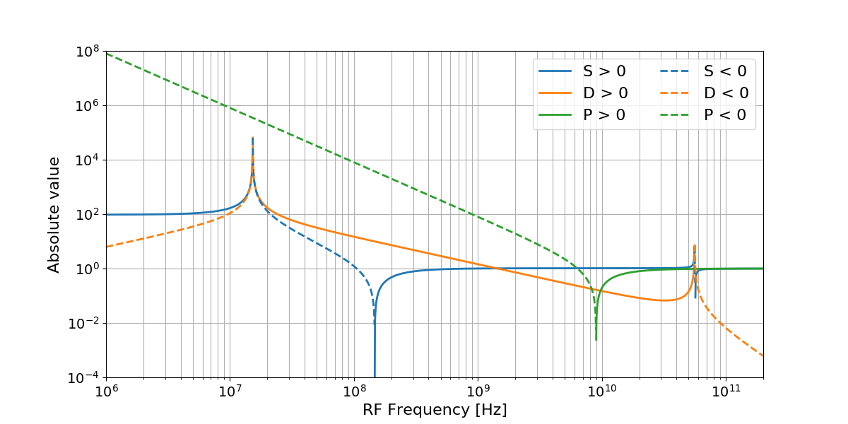
Filter positive and negative values, for display purposes only. Still for display purposes, replace 0 by NaN to NOT plot 0 values

S_pos = S * (S > 0)
D_pos = D * (D > 0)
P_pos = P * (P > 0)
S_neg = S * (S < 0)
D_neg = D * (D < 0)
P_neg = P * (P < 0)
S_pos[S_pos == 0] = np.NaN
D_pos[D_pos == 0] = np.NaN
P_pos[P_pos == 0] = np.NaN
S_neg[S_neg == 0] = np.NaN
D_neg[D_neg == 0] = np.NaN
P_neg[P_neg == 0] = np.NaN

plt.figure(figsize=(12, 6))
plt.semilogx(f, abs(S_pos),
             f, abs(D_pos),
             f, abs(P_pos), lw=2)
plt.semilogx(f, abs(S_neg), '#1f77b4',
             f, abs(D_neg), '#ff7f0e',
             f, abs(P_neg), '#2ca02c', lw=2, ls='--')
plt.yscale('log')
plt.grid(True, which='major')
plt.grid(True, which='minor')
plt.ylim(1e-4, 1e8)
plt.xlim(1e6, 200e9)
plt.legend(('S > 0', 'D > 0', 'P > 0', 'S < 0', 'D < 0', 'P < 0'),
           fontsize=16, ncol=2)
plt.xlabel('RF Frequency [Hz]', size=16)
plt.ylabel('Absolute value', size=16)
plt.tick_params(labelsize=14)

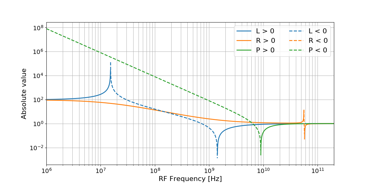
Cold Plasma tensor elements in the rotating basis

L, R, P = pp.physics.cold_plasma_permittivity_LRP(B, species, n, omega_RF)

L_pos = L * (L > 0)
R_pos = R * (R > 0)
L_neg = L * (L < 0)
R_neg = R * (R < 0)
L_pos[L_pos == 0] = np.NaN
R_pos[R_pos == 0] = np.NaN
L_neg[L_neg == 0] = np.NaN
R_neg[R_neg == 0] = np.NaN

plt.figure(figsize=(12, 6))
plt.semilogx(f, abs(L_pos),
             f, abs(R_pos),
             f, abs(P_pos), lw=2)
plt.semilogx(f, abs(L_neg), '#1f77b4',
             f, abs(R_neg), '#ff7f0e',
             f, abs(P_neg), '#2ca02c', lw=2, ls='--')
plt.yscale('log')
plt.grid(True, which='major')
plt.grid(True, which='minor')
plt.xlim(1e6, 200e9)
plt.legend(('L > 0', 'R > 0', 'P > 0', 'L < 0', 'R < 0', 'P < 0'),
           fontsize=16, ncol=2)
plt.xlabel('RF Frequency [Hz]', size=16)
plt.ylabel('Absolute value', size=16)
plt.tick_params(labelsize=14)

Checks if the values obtained are coherent. They should satisfy S = (R+L)/2 and D = (R-L)/2

try:
    np.testing.assert_allclose(S, (R + L) / 2)
    np.testing.assert_allclose(D, (R - L) / 2)
except AssertionError as e:
    print(e)
# Checks for R=S+D and L=S-D
try:
    np.testing.assert_allclose(R, S + D)
    np.testing.assert_allclose(L, S - D)
except AssertionError as e:
    print(e)

Total running time of the script: ( 0 minutes 0.192 seconds)