Analysing ITER parameters

Let’s try to look at ITER plasma conditions using the physics subpackage.

from astropy import units as u
from plasmapy import physics
import matplotlib.pyplot as plt
import numpy as np
from mpl_toolkits.mplot3d import Axes3D

The radius of electric field shielding clouds, also known as the Debye length, would be

electron_temperature = 8.8 * u.keV
electron_concentration = 10.1e19 / u.m**3
print(physics.Debye_length(electron_temperature, electron_concentration))

Out:

6.939046841173439e-05 m

Note that we can also neglect the unit for the concentration, as 1/m^3 is the a standard unit for this kind of Quantity:

print(physics.Debye_length(electron_temperature, 10.1e19))

Out:

6.939046841173439e-05 m

Assuming the magnetic field as 5.3 Teslas (which is the value at the major radius):

B = 5.3 * u.T

print(physics.gyrofrequency(B, particle='e'))

print(physics.gyroradius(B, T_i=electron_temperature, particle='e'))

Out:

932174612509.1257 rad / s
5.968562743414285e-05 m

The electron inertial length would be

print(physics.inertial_length(electron_concentration, particle='e'))

Out:

0.0005287720431268747 m

In these conditions, they should reach thermal velocities of about

print(physics.thermal_speed(T=electron_temperature, particle='e'))

Out:

55637426.625786155 m / s

And the Langmuir wave plasma frequency should be on the order of

print(physics.plasma_frequency(electron_concentration))

Out:

566959736046.5352 rad / s

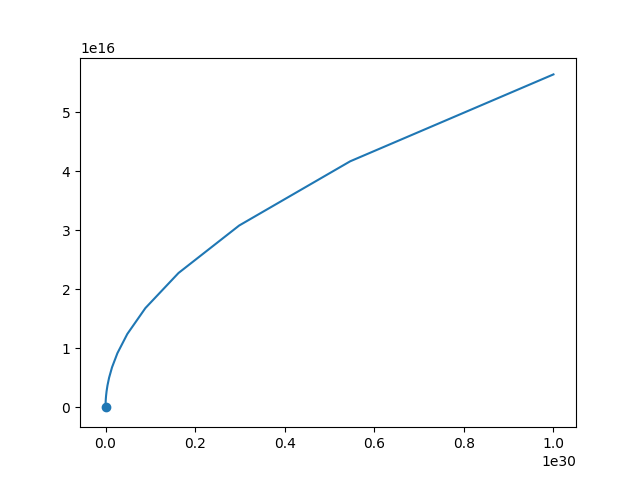
Let’s try to recreate some plots and get a feel for some of these quantities.

n_e = np.logspace(4, 30, 100) / u.m**3
plt.plot(n_e, physics.plasma_frequency(n_e))
plt.scatter(
    electron_concentration,
    physics.plasma_frequency(electron_concentration))

Total running time of the script: ( 0 minutes 0.324 seconds)