The plasma dispersion function

Let’s import some basics (and PlasmaPy!)

import numpy as np
import matplotlib.pyplot as plt
import plasmapy

help(plasmapy.mathematics.plasma_dispersion_func)

Out:

Help on function plasma_dispersion_func in module plasmapy.mathematics.mathematics:

plasma_dispersion_func(zeta:Union[complex, int, float, numpy.ndarray]) -> Union[complex, float, numpy.ndarray]
    Calculate the plasma dispersion function.

    Parameters
    ----------
    zeta : complex, int, float, ~numpy.ndarray, or ~astropy.units.Quantity
        Argument of plasma dispersion function.

    Returns
    -------
    Z : complex, float, or ~numpy.ndarray
        Value of plasma dispersion function.

    Raises
    ------
    TypeError
        If the argument is of an invalid type.

    ~astropy.units.UnitsError
        If the argument is a `~astropy.units.Quantity` but is not
        dimensionless.

    ValueError
        If the argument is not entirely finite.

    See Also
    --------
    plasma_dispersion_func_deriv

    Notes
    -----
    The plasma dispersion function is defined as:

    .. math::
        Z(\zeta) = \pi^{-0.5} \int_{-\infty}^{+\infty}
        \frac{e^{-x^2}}{x-\zeta} dx

    where the argument is a complex number [fried.conte-1961]_.

    In plasma wave theory, the plasma dispersion function appears
    frequently when the background medium has a Maxwellian
    distribution function.  The argument of this function then refers
    to the ratio of a wave's phase velocity to a thermal velocity.

    References
    ----------
    .. [fried.conte-1961] Fried, Burton D. and Samuel D. Conte. 1961.
       The Plasma Dispersion Function: The Hilbert Transformation of the
       Gaussian. Academic Press (New York and London).

    Examples
    --------
    >>> plasma_dispersion_func(0)
    1.7724538509055159j
    >>> plasma_dispersion_func(1j)
    0.757872156141312j
    >>> plasma_dispersion_func(-1.52+0.47j)
    (0.6088888957234254+0.33494583882874024j)

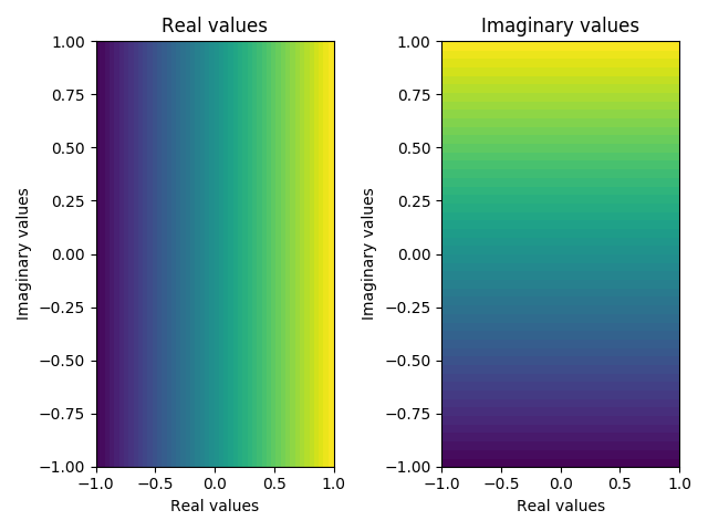
We’ll now make some sample data to visualize the dispersion function:

x = np.linspace(-1, 1, 1000)
X, Y = np.meshgrid(x, x)
Z = X + 1j * Y
print(Z.shape)

Out:

(1000, 1000)

Before we start plotting, let’s make a visualization function first:

def plot_complex(X, Y, Z, N=50):
    fig, (real_axis, imag_axis) = plt.subplots(1, 2)
    real_axis.contourf(X, Y, Z.real, N)
    imag_axis.contourf(X, Y, Z.imag, N)
    real_axis.set_title("Real values")
    imag_axis.set_title("Imaginary values")
    for ax in [real_axis, imag_axis]:
        ax.set_xlabel("Real values")
        ax.set_ylabel("Imaginary values")
    fig.tight_layout()


plot_complex(X, Y, Z)

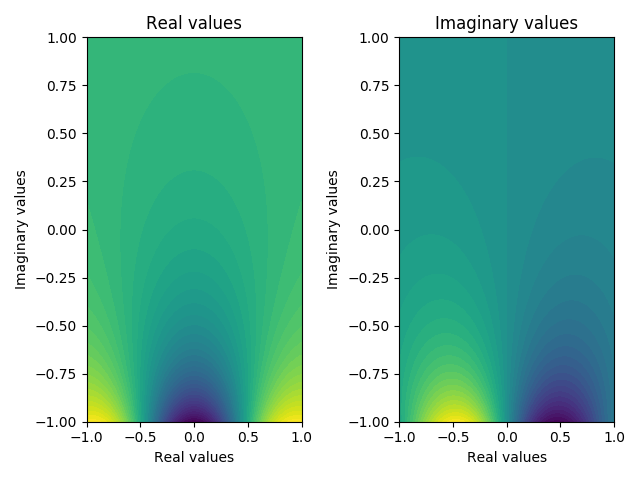
We can now apply our visualization function to our simple

F = plasmapy.mathematics.plasma_dispersion_func(Z)
plot_complex(X, Y, F)

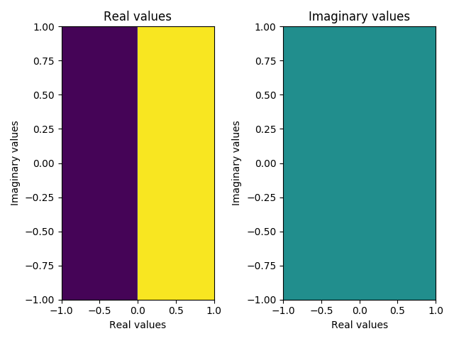
So this is going to be a hack and I’m not 100% sure the dispersion function is quite what I think it is, but let’s find the area where the dispersion function has a lesser than zero real part because I think it may be important (brb reading Fried and Conte):

plot_complex(X, Y, F.real < 0)

We can also visualize the derivative:

F = plasmapy.mathematics.plasma_dispersion_func_deriv(Z)
plot_complex(X, Y, F)

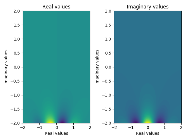
Plotting the same function on a larger area:

x = np.linspace(-2, 2, 2000)
X, Y = np.meshgrid(x, x)
Z = X + 1j * Y
print(Z.shape)

Out:

(2000, 2000)

F = plasmapy.mathematics.plasma_dispersion_func(Z)
plot_complex(X, Y, F, 100)

Total running time of the script: ( 0 minutes 23.300 seconds)