1D Maxwellian distribution function

We import the usual and the hero of this notebook, the Maxwellian 1D distribution:

import numpy as np
from astropy import units as u
import plasmapy
import matplotlib.pyplot as plt
from plasmapy.constants import (m_p, m_e, c, mu0, k_B, e, eps0, pi, e)
from plasmapy.physics.distribution import Maxwellian_1D

Given we’ll be plotting:

from astropy.visualization import quantity_support
quantity_support()

Let’s get the probability density of finding an electron at 1 m/s if we have a plasma at 30 000 K:

Maxwellian_1D(
    v=1 * u.m / u.s,
    T=30000 * u.K,
    particle='e',
    V_drift=0 * u.m / u.s)

Note the units! Integrated over velocities, this will give us a probability. Let’s test that for a bunch of particles:

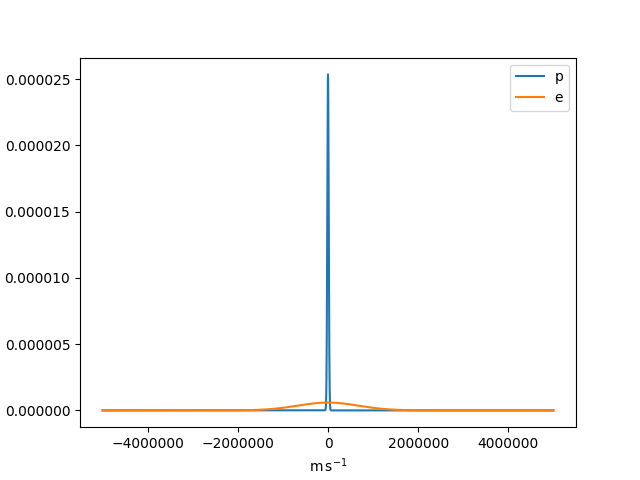
With a vector (from Numpy)

start = -500000
stop = -start
v = np.arange(start, stop) * 10 * u.m / u.s
dv = v[1] - v[0]

Test the normalization to 1 (the particle has to be somewhere)

for particle in ['p', 'e']:
    pdf = Maxwellian_1D(v, T=30000 * u.K, particle=particle)
    integral = (pdf).sum() * dv
    print(f"Integral value for {particle}: {integral}")
    plt.plot(v, pdf, label=particle)
plt.legend()

Out:

Integral value for p: 0.9999999999999999
Integral value for e: 0.9999999999998787

The standard deviation of this distribution should give us back our temperature:

T = 30000 * u.K
std = np.sqrt((Maxwellian_1D(v, T=T, particle='e') * v**2 * dv).sum())
T_theo = (std**2 / k_B * m_e).to(u.K)

print(T_theo / T)

Out:

0.9999999999930749

And the center of the distribution is, as can be seen below:

T_e = 30000 * u.K
V_drift = 10 * u.km / u.s

start = -5000
stop = - start
dv = 10000 * u.m / u.s

v_vect = np.arange(start, stop, dtype='float64') * dv

print(v_vect[Maxwellian_1D(v_vect, T=T_e,
                           particle='e', V_drift=V_drift).argmax()])

Out:

10000.0 m / s

Total running time of the script: ( 0 minutes 1.083 seconds)